P1, The Stroop effect
This will be the first post I fully dedicate to one of the Udacity Data Analysis Nanodegree projects. For this project I decided to use excel for analysis and visualizations in order to be able to focus on the process and writing rather than the tools.
In this post, we will take a look at a classic phenomenon from experimental psychology, the Stroop effect. After a short description of the effect, we will present some data and then proceed with calculating statistics and performing a test to see if there are any difference in response time while naming colors from two different predefined lists out loud.
Background
The effect is named after an American psychologist named John Ridley Stroop. His findings were published in 1935. The Stroop effect is showcasing the interference in reaction times demonstrated by subjects naming colors listed in two different types of lists. In the first list, the color of the font is the same as the color written. In the second list, the font and written colors are different. The test subject needs to say out loud the color of the font. From here on, the first list will be described as congruent and the second list as incongruent.
Variables, Hypotheses, and Test type
We will proceed by doing a statistical test to see if the reading time is changed significantly between the two types of lists using a small sample of data. We start by defining our variables for the test.
The independent variable is the type of list, which we change in between the two times the test subject performs the test. The dependent variable is the measured time to complete reading through each of the lists.
We are interested in seeing if the dependent variable (measured time) is affected by our independent variable (type of list) and therefore define the below two hypotheses based on the population mean $ \mu $ for congruent($ c $) and incongruent ($ i $) list reading time:
(The measured reading time is unchanged between list types)
(The measured reading time do change between list types)
Since we won’t have any access to information about the population as a whole, just two rather small samples, we will perform a t-test suitable for this sample size. We will use the standard deviation and mean of our sample to evaluate if there is any statistically significant change between the two reading times. With a larger sample size and data about the population standard deviation, we could have opted for a z-test instead.
By choosing to do a t-test we make the following assumptions about our test data:
- The reading time are randomly sampled from the whole population.
- The reading time is normally distributed when looking at the population as a whole.
- The values for our sample data follow a continuous scale.
Further, for a paired sample t-test the following assumptions are made as well:
- Just as the original reading times are, the difference in seconds between the two reading times are also normally distributed.
- The two samples are linked with each other due to the measurement being repeated two times for each subject.
Source for the t-test assumptions can be found here.
We will compare two samples (measured time) where each test subject are present in both samples (once for the congruent and once more for the incongruent list), so the sample data sets will be dependent on each other. This means we can perform a paired sample t-test where we look at the difference between the two list types reading times. This will gives us the following equations for our t-statistic($ t_{statistic} $) and degrees of freedom($ df $):
$ X $ is the mean of the sample for the congruent($ c $) and incongruent($ i $) lists reading times, $ S $ is the standard deviation for the differences in reading times between the two list types in our sample, and $ n $ is the sample size.
Data
To be able to perform any calculations the following existing data set will be used. I have added my own times to the two lists on the last row and also calculated the differences in reading time as written in the third column. If you are curious about the test yourself, please feel free to check it out via this link.
Reading times (in seconds)
| Congruent $( X_c ) $ | Incongruent $( X_i )$ | Difference $( X_d = X_i - X_c )$ |
|---|---|---|
| 12.079 | 19.278 | 7.199 |
| 16.791 | 18.741 | 1.950 |
| 9.564 | 21.214 | 11.65 |
| 8.630 | 15.687 | 7.057 |
| 14.669 | 22.803 | 8.134 |
| 12.238 | 20.878 | 8.640 |
| 14.692 | 24.572 | 9.880 |
| 8.987 | 17.394 | 8.407 |
| 9.401 | 20.762 | 11.361 |
| 14.480 | 26.282 | 11.802 |
| 22.328 | 24.524 | 2.196 |
| 15.298 | 18.644 | 3.346 |
| 15.073 | 17.510 | 2.437 |
| 16.929 | 20.330 | 3.401 |
| 18.200 | 35.255 | 17.055 |
| 12.130 | 22.158 | 10.028 |
| 18.495 | 25.139 | 6.644 |
| 10.639 | 20.429 | 9.790 |
| 11.344 | 17.425 | 6.081 |
| 12.369 | 34.288 | 21.919 |
| 12.944 | 23.894 | 10.950 |
| 14.233 | 17.960 | 3.727 |
| 19.710 | 22.058 | 2.348 |
| 16.004 | 21.157 | 5.153 |
| 11.940 | 15.650 | 3.710 |
From the above data we are also able to calculate following descriptive measurements:
(Mean reading time for the congruent list)
(Mean reading time for the _incongruent_ list)
(Estimated standard deviation for the time difference between $ X_c $ and $ X_i $)
(Sample size)
Visual analysis
Before we start the testing let’s have a look at our data to see if there is something we have missed. We begin with a simple histogram showing the number of occurrences for different reading times.
Reading times (occurrences)
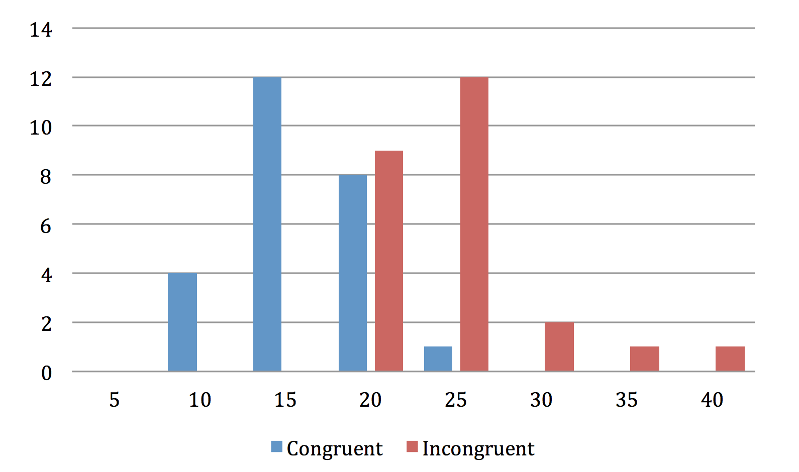
Judging from the above plot it does seem like the incongruent list type increases the reading time, but we will wait until a little bit later to see if the observed difference in our samples has any statistical significance. For now, I believe it is okay to just observe that both shapes look to be bell-shaped and that we will not have any trouble proceeding with our planned t-test.
List reading time distribution
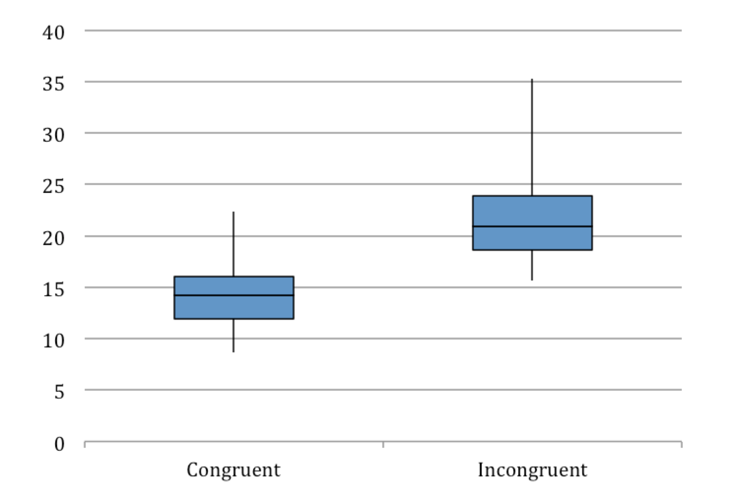
Another way to visualize the data is to use a box plot, as seen above. Here once again we see that the reading times for the incongruent list are increased in comparison to the congruent list. Compared to the previous bin plot we can see that there is less overlap between the two sample groups for values in the 15- to 20-second interval than one might first think. The reason being that most of the reading times for the congruent list is in the lower and while the incongruent list times are in the higher end of the interval of the bin in the previous plot.
t-Test and conclusion
Now let’s proceed by testing our hypotheses with a double-sided t-test at a confidence level of 95%. Together with the information we have gathered so far, the confidence level gives us the following degrees of freedom and critical value for $ t $.
To continue, we input the measures we obtained from our data into the equation for our $ t_{statistic} $ and get the following results:
(with)
Since $ t_{statistic} > t_{critical} $ we reject the null hypothesis, there is a significant change in reading time between the two list types.
I believe this comes as no surprise if you tried the test yourself with the link provided at the beginning of this post. There is a noticeable difference in the concentration necessary for reading the second incongruent word list in comparison with the first congruent list. But now we can back up our own hunch with data and draw the conclusion that it isn’t only us that experiences this difference.
As why this is the case I can only speculate, but after a quick visit to Wikipedia and some reading it seems that one possible explanation is that both the font color and the written color are being processed at the same time in the brain causing the two signals to interfere with each other influencing the response time and failure rate.