P2, Surviving Titanic
This is the second post dedicated to my Udacity nanodegree and this time the project is my first go at doing a full data analysis from start to finish using Python notebook and pandas (together with scipy and statsmodels). To give focus to the overarching process I have made some choices in order to simplify the analysis, as you will see. I am planning to give more focus on the data wrangling, model building, and visualization/communication phases in upcoming posts.
Introduction and initial questions
This time we will take a look at a dataset containing passenger information from the Titanic and see if we can find any patterns in the data pointing to if sex, age or social status had any influence over the probability of surviving the disastrous shipwreck.
Was it possibly so that the upper class were favored and had a higher chance of survival than the other passengers? Perhaps age made a difference? And was it really ladies first, even for a place on a lifeboat on the sinking ship?
We will take a look at and analyze the dataset to see if we can find the answers to these questions. But first, before we start let’s import the libraries we will need for our analysis.
# Importing numpy and pandas for handy data handling.
import numpy as np
import pandas as pd

# Matplotlib for plotting our data and seaborn for styling our plots.
import matplotlib.pyplot as plt
import seaborn

# Importing chi square test from scipy.stats package to test for independence
from scipy.stats import chi2_contingency

# We will use statsmodels logistic regression model to analyze
# the different probabilities of survival depending on age, gender, and class.
import statsmodels.api as sm

# Enabling inline plots.
%matplotlib inline
Now we are ready to tackle our chosen dataset.
The dataset
The set itself is taken from the following Kaggle competition which works as an introduction to their machine learning competitions. We will use the same dataset but will focus more on our analysis of the data rather than making predictions of who will live or die.
We start by reading in the data using the pandas CSV reader and take a look at what we have to play with.
passengers = pd.read_csv('titanic-data.csv')
passengers.head(3)
| PassengerId | Survived | Pclass | Name | Sex | Age | SibSp | Parch | Ticket | Fare | Cabin | Embarked | |
|---|---|---|---|---|---|---|---|---|---|---|---|---|
| 0 | 1 | 0 | 3 | Braund, Mr. Owen Harris | male | 22.0 | 1 | 0 | A/5 21171 | 7.2500 | NaN | S |
| 1 | 2 | 1 | 1 | Cumings, Mrs. John Bradley (Florence Briggs Th… | female | 38.0 | 1 | 0 | PC 17599 | 71.2833 | C85 | C |
| 2 | 3 | 1 | 3 | Heikkinen, Miss. Laina | female | 26.0 | 0 | 0 | STON/O2. 3101282 | 7.9250 | NaN | S |
It seems like the data has been read without any major problems, but there are some columns in the given set that might need further explanation. The following explanations are given on the Kaggle competition page.
| Variable | Definition | Key |
|---|---|---|
| survival | Survival | 0 = No, 1 = Yes |
| pclass | Ticket class | 1 = 1st, 2 = 2nd, 3 = 3rd |
| sex | Sex | |
| Age | Age in years | |
| sibsp | # of siblings / spouses aboard the Titanic | |
| parch | # of parents / children aboard the Titanic | |
| ticket | Ticket number | |
| fare | Passenger fare | |
| cabin | Cabin number | |
| embarked | Port of Embarkation | C = Cherbourg, Q = Queenstown, S = Southampton |
We can also see that there are some ‘NaN’ values present in the cabin column so
we will take an extra look at our data with the .info() method to see how many
missing values there are.
# Check info about the data we read with .read_csv()
passengers.info()
# Output
<class 'pandas.core.frame.DataFrame'>
RangeIndex: 891 entries, 0 to 890
Data columns (total 12 columns):
PassengerId    891 non-null int64
Survived       891 non-null int64
Pclass         891 non-null int64
Name           891 non-null object
Sex            891 non-null object
Age            714 non-null float64
SibSp          891 non-null int64
Parch          891 non-null int64
Ticket         891 non-null object
Fare           891 non-null float64
Cabin          204 non-null object
Embarked       889 non-null object
dtypes: float64(2), int64(5), object(5)
memory usage: 83.6+ KB
We can see that in addition to the Cabin column, Age, and Embarked columns are also missing values. We either need to estimate these missing values or drop them.
We could estimate missing ages with either median or average values, but for our analysis, the non-null 714 values will be enough. We choose to just drop the rows with null values. Cabin has too many missing values to make anything out of and according to Wikipedia also a possible bias towards first class passengers. However, something that would be interesting to look up another time is for example if cabin proximity to the few lifeboats that were available influenced the possibility of survival. This is out of scope so instead, we choose to just drop the columns.
Also, upon further inspection, it seems like SibSp/Parch and ticket numbers don’t have much of a connection making it hard to make sense of which passengers are related to who. There might be some interesting analysis in answering the question if being in a group increased or decreased the probability of survival. But, once again this might be a bit to much work for this time so we choose to drop these three columns as well.
The same reasoning goes for the Name, PassengerId, and Fare columns which we all choose to drop.
# Dropping rows with NaN values
passengers.dropna(subset=['Age'], inplace=True)

# Dropping unneeded columns
passengers.drop('Cabin', axis=1, inplace=True)
passengers.drop('Embarked', axis=1, inplace=True)

passengers.drop('SibSp', axis=1, inplace=True)
passengers.drop('Parch', axis=1, inplace=True)
passengers.drop('Ticket', axis=1, inplace=True)

passengers.drop('Name', axis=1, inplace=True)
passengers.drop('PassengerId', axis=1, inplace=True)
passengers.drop('Fare', axis=1, inplace=True)
Lastly, to make column names more coherent we rename the Pclass column to just Class and to better describe to contents of each column we convert the Sex, Class, and Survived column’s data types from Strings to Categories, and Integers to booleans.
passengers = passengers.rename(columns={'Pclass': 'Class'})

passengers['Sex'] = passengers['Sex'].astype('category')
passengers['Class'] = passengers['Class'].astype('category')

passengers['Survived'] = passengers['Survived'].apply(bool)
This gives us the below data frame to work with.
passengers.head()
| Survived | Class | Sex | Age | |
|---|---|---|---|---|
| 0 | False | 3 | male | 22.0 |
| 1 | True | 1 | female | 38.0 |
| 2 | True | 3 | female | 26.0 |
| 3 | True | 1 | female | 35.0 |
| 4 | False | 3 | male | 35.0 |
passengers.info()
# Output
<class 'pandas.core.frame.DataFrame'>
Int64Index: 714 entries, 0 to 890
Data columns (total 4 columns):
Survived    714 non-null bool
Class       714 non-null category
Sex         714 non-null category
Age         714 non-null float64
dtypes: bool(1), category(2), float64(1)
memory usage: 13.3 KB
Descriptive stats
To get a better grip of the data we use the pandas dataframe’s .describe()
method to see some statistics describing each of the variables in our dataset.
passengers['Age'].describe()
# Output
count    714.000000
mean      29.699118
std       14.526497
min        0.420000
25%       20.125000
50%       28.000000
75%       38.000000
max       80.000000
Name: Age, dtype: float64
passengers['Sex'].describe()
# Output
count      714
unique       2
top       male
freq       453
Name: Sex, dtype: object
passengers['Class'].describe()
# Output
count     714
unique      3
top         3
freq      355
Name: Class, dtype: int64
passengers['Survived'].describe()
# Output
count       714
unique        2
top       False
freq        424
Name: Survived, dtype: object
Based on the above, we can see that for our sample the typical passenger was a male around 30 traveling in third class and, unfortunately, did not survive the shipwreck. Worth noting is that after we cleaned up the data we have no missing values in any of our remaining columns.
Let’s try to plot some different relationships between class, sex, and age for the survivors and non-survivors in our data set to see if we can find something interesting. We start out with plotting comparisons for the composition of passenger class and sex between survivors and casualties.
# Create a grid with two columns for display
fig, axs = plt.subplots(ncols=2, figsize=(12, 4))

# Pivot passengers by Survived and Class then plot the results in a bar graph
survived_by_class = pd.pivot_table(data=passengers[['Survived', 'Class']], \
                                  index='Survived', \
                                  columns=['Class'], \
                                  aggfunc=len)

survived_by_class.plot(kind='bar', stacked=True, ax=axs[0])
axs[0].set(title='1. Survivors by Class', ylabel='Passengers')

# Do the same as above but with Survived and Sex
survived_by_sex = pd.pivot_table(data=passengers[['Survived', 'Sex']], \
                                 index='Survived', \
                                 columns=['Sex'], \
                                 aggfunc=len)

survived_by_sex.plot(kind='bar', stacked=True, ax=axs[1])
axs[1].set(title='2. Survivors by Sex', ylabel='Passengers')

# Display plots
plt.show()
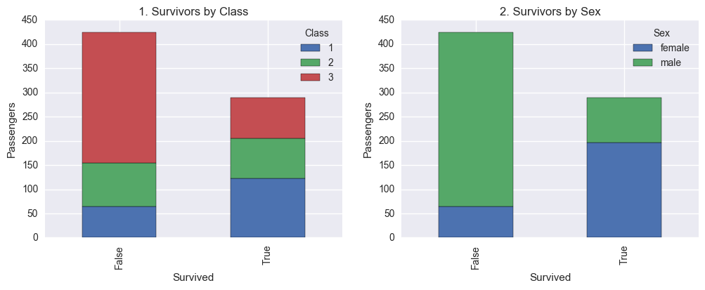
From the above bar graphs we can see that there is a big change in the ratio between male and female, and between third class and first/second class passengers represented in the two different categories (Survived: False/True). It does look as if women had a higher chance of survival than men and third class passengers a much lower chance than 1 class passengers. To really make sure that this isn’t just in our sample we will perform two tests to see if the deviations are statistically significant or not.
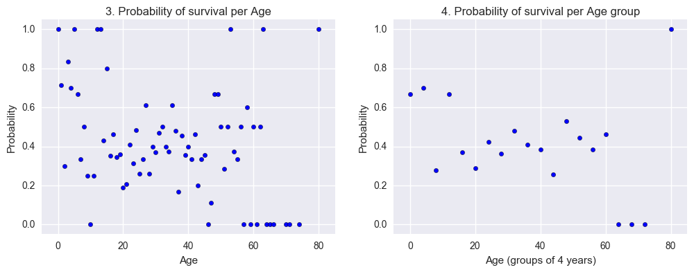
We also tried plotting the survival rate for passengers born the same year but too much noise makes it hard to draw any conclusions from it. By combining ages into intervals of 4 we can keep some of the noise down. Judging from the adjusted graph it looks like we might have a correlation between higher age and a decreased probability of survival. We will also try to answer this question later on using logistic regression.
# Create a new grid for plots
fig, axs = plt.subplots(ncols=2, figsize=(12, 4))

#Grouped and plotted by age in full years
survival_by_age = passengers.groupby(lambda x: int(passengers.loc[x].Age)).Survived
survival_rate_by_age = survival_by_age.apply(lambda x: x[x == True].count()/(x.count() * 1.0))
axs[0].scatter(survival_rate_by_age.index, survival_rate_by_age);
axs[0].set(title='3. Probability of survival per Age',
           xlabel='Age',
           ylabel='Probability',
           xlim=[-5, 85],
           ylim=[-0.05,1.05])

#Grouped and plotted by age in intervals of 4
survival_by_age_group = passengers.groupby(lambda x: int(passengers.loc[x].Age/4)*4).Survived
survival_rate_by_age_group = survival_by_age_group.apply(lambda x: x[x == True].count()/(x.count() * 1.0))
axs[1].scatter(survival_rate_by_age_group.index, survival_rate_by_age_group);
axs[1].set(title='4. Probability of survival per Age group',
           xlabel='Age (groups of 4 years)',
           ylabel='Probability',
           xlim=[-5, 85],
           ylim=[-0.05,1.05]);
Chi-squared test for independence
To summarize, after looking at the above three variables and plots we can hypothesize about there being three factors that all had an effect on the chance of survival.
- Class, third class passengers had a lower probability of survival than first and second class passengers.
- Sex, women had a higher probability of survival than men.
- Age, higher age meant a decreased chance of survival.
We will start by using a chi squared test for independence to test if the survival for our passengers are dependent on our first two factors, Class and Gender.
The test is possible to perform since all our involved variables are categorical, meaning that all our outcomes are mutually exclusive (you cannot be dead and alive, or in first and second class at the same time) and the total probability of all outcomes adds up to 1 (meaning you have to be either be dead or alive etc).
Explained very shortly to do a chi-squared test we calculate our chi-square statistic, $\chi^2$, as a normalized sum of the squared deviations between observed and expected frequencies and then compare the statistic to a critical value (found in a table) based on our chosen confidence level and the degrees of freedom. Expressed mathematically it looks something like the below.
where
$\chi^2 =$ The chi square statistic
$O_i =$ Observations of type i
$E_i = Np_i =$ expected frequency for type i
$N =$ Total number of observations
$n =$ Number of types of observations
To test for variable independence we formulate the following hypothesis.
$H_0$: The variables are independent.
$H_a$: The variables are not independent.
We start with testing survival and class to see if class did have a statistically significant effect on survival. We are using the same pivot table we used to display our bar plot earlier as input.
survived_by_class
| Class | 1 | 2 | 3 |
|---|---|---|---|
| Survived | |||
| False | 64 | 90 | 270 |
| True | 122 | 83 | 85 |
chi2, p_value, dof, expected = chi2_contingency(survived_by_class)

print 'Degrees of freedom: ' + str(dof)
print 'Chi squared test score: ' + str(chi2)
print 'P-value: ' + str(p_value)
# Output
Degrees of freedom: 2
Chi squared test score: 92.9014172114
P-value: 6.70986174976e-21
Looking up the critical value in a $\chi^2$-table we see that the value of our statistic is higher than all values given for 2 degrees of freedom. This means that there is a dependence between survival and class significant for all reasonable $\alpha$. As a result, we reject our $H_0$.
Similarly, for survival and sex we use our old pivot table and receive the following results.
survived_by_sex
| Sex | female | male |
|---|---|---|
| Survived | ||
| False | 64 | 360 |
| True | 197 | 93 |
chi2, p_value, dof, expected = chi2_contingency(survived_by_sex)

print 'Degrees of freedom: ' + str(dof)
print 'Chi squared test score: ' + str(chi2)
print 'P-value: ' + str(p_value)
# Output
Degrees of freedom: 1
Chi squared test score: 205.025827529
P-value: 1.67166784414e-46
Once again we get a statistic value larger than any critical value for any reasonable $\alpha$. We once again reject $H_0$ and conclude that there is a significant dependency between sex and the probability for survival.
Logistical regression for probabilities
Next, we will take our analysis one step further and investigate the relation between age and survival with help from the logistical regression model from the statsmodels package. For a more extensive example have a look at this blog post which I also used as a reference for the following analysis.
Since we already have verified that both class and sex also influences survival we choose to add these variables as well to our regression model. In order to add these two non-continuous variables we need to create some additional dummy variables to represent the different values for class and age as simple True(1) or False(0) variables. This is simple to do using pandas .get_dummies() method.
# Add dummy variables for class and sex.
passenger_dummies = passengers.join(
    pd.get_dummies(passengers['Class'], prefix='Class'))
passenger_dummies = passenger_dummies.join(
    pd.get_dummies(passengers['Sex']))

# We drop the Class and Sex columns from the table since they aren't needed.
passenger_dummies.drop('Class', axis=1, inplace=True)
passenger_dummies.drop('Sex', axis=1, inplace=True)

# To create a baseline, our typical passenger, we drop the class 3 and male column.
passenger_dummies.drop('Class_3', axis=1, inplace=True)
passenger_dummies.drop('male', axis=1, inplace=True)

passenger_dummies.head()
| Survived | Age | Class_1 | Class_2 | female | |
|---|---|---|---|---|---|
| 0 | False | 22.0 | 0 | 0 | 0 |
| 1 | True | 38.0 | 1 | 0 | 1 |
| 2 | True | 26.0 | 0 | 0 | 1 |
| 3 | True | 35.0 | 1 | 0 | 1 |
| 4 | False | 35.0 | 0 | 0 | 0 |
Next step is to feed our data into the logistic regression model from the statsmodel package and fit it to the inputted data.
logit = sm.Logit(passenger_dummies['Survived'],
                 passenger_dummies[passenger_dummies.columns[1:]])

# Fit the model
result = logit.fit()

result.summary()
# Output
Optimization terminated successfully.
        Current function value: 0.474695
        Iterations 6
Logit regression results
| Dep. Variable: | Survived | No. Observations: | 714 |
| Model: | Logit | Df Residuals: | 710 |
| Method: | MLE | Df Model: | 3 |
| Date: | Sun, 07 May 2017 | Pseudo R-squ.: | 0.2972 |
| Time: | 20:23:52 | Log-Likelihood: | -338.93 |
| converged: | True | LL-Null: | -482.26 |
| LLR p-value: | 7.700e-62 |
| coef | std err | z | P>z | [0.025 | 0.975] | |
|---|---|---|---|---|---|---|
| Age | -0.0682 | 0.006 | -12.145 | 0.000 | -0.079 | -0.057 |
| Class_1 | 2.6026 | 0.283 | 9.196 | 0.000 | 2.048 | 3.157 |
| Class_2 | 0.9867 | 0.233 | 4.232 | 0.000 | 0.530 | 1.444 |
| female | 2.1893 | 0.198 | 11.035 | 0.000 | 1.800 | 2.578 |
Looking at the coefficient for Age, we can see that there is a negative relation between passenger age and the probability of survival. On the other hand Class_1, Class_2, and female have positive coefficients meaning that there is a positive correlation between both passenger class and sex, and the probability of survival. This confirms our chi^2 test results and the initial hypothesis that more women and higher class passengers had a higher probability of survival.
It is also important to note that the confidence intervals for all coefficients are strictly negative or strictly positive meaning there is a significant probability that each of the coefficients have influence over passengers chance of survival.
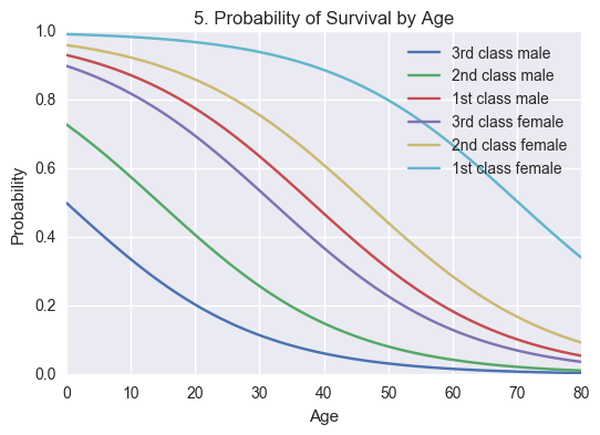
As a last trick, we plot all the different possibilities for survival based on age for each combination of our categorical variables so that we can visualize what passengers had the highest and/or lowest possibility of survival for the shipwreck.
# Last step, visualizing the probability for all possible data points
ages = np.linspace(0, 80, 81, dtype=int)

# Define cartesian function
def cartesian(arrays, out=None):
    arrays = [np.asarray(x) for x in arrays]
    dtype = arrays[0].dtype

    n = np.prod([x.size for x in arrays])
    if out is None:
        out = np.zeros([n, len(arrays)], dtype=dtype)

    m = n / arrays[0].size
    out[:,0] = np.repeat(arrays[0], m)
    if arrays[1:]:
        cartesian(arrays[1:], out=out[0:m,1:])
        for j in xrange(1, arrays[0].size):
            out[j*m:(j+1)*m,1:] = out[0:m,1:]
    return out

# Enumerate all possible combinations of dummy variables (0=male, 1=female)
combinations = pd.DataFrame(cartesian([ages, [1, 2, 3], [0, 1]]))

# Recreate dummies
combinations.columns = ['age', 'class', 'female']

dummy_classes = pd.get_dummies(combinations['class'])
dummy_classes.columns = ['class_1', 'class_2', 'class_3']

dummy_sexes = pd.get_dummies(combinations['female'])
dummy_sexes.columns = ['male', 'female']

# Keep what we need for predictions and join with combinations
combinations = pd.DataFrame(combinations['age']).join(dummy_classes.ix[:, :'class_2'])
combinations = combinations.join(dummy_sexes.ix[:, 'female':])

combinations['survival_prediction'] = result.predict(combinations)

# Predicted survival probabilities for an average age passenger.
combinations[180:186]
| age | class_1 | class_2 | female | survival_prediction | |
|---|---|---|---|---|---|
| 180 | 30 | 1 | 0 | 0 | 0.635962 |
| 181 | 30 | 1 | 0 | 1 | 0.939755 |
| 182 | 30 | 0 | 1 | 0 | 0.257695 |
| 183 | 30 | 0 | 1 | 1 | 0.756086 |
| 184 | 30 | 0 | 0 | 0 | 0.114586 |
| 185 | 30 | 0 | 0 | 1 | 0.536085 |
#Pivoting table for plotting.
pivot = pd.pivot_table(combinations,
                       values=['survival_prediction'],
                       index=['age'],
                       columns=['female', 'class_1', 'class_2'])

# And plot the resulting graph.
fig, ax = plt.subplots()
pivot.plot(title='5. Probability of Survival by Age',
           ax=ax)
ax.set(xlabel='Age', ylabel='Probability')

# Giving the legend some readable labels.
lines, labels = ax.get_legend_handles_labels()
ax.legend(lines, ['3rd class male',
                  '2nd class male',
                  '1st class male',
                  '3rd class female',
                  '2nd class female',
                  '1st class female',]);
Conclusion
From the last plot, we can see that our analysis shows a relation between higher age and a lower chance of surviving the shipwreck for all classes and sexes. Further, the different combinations of passenger sex and class can be ranked the following way, from highest probability of survival to lowest compared to other passengers of the same age. (Color from above plot in brackets)
- First class women (Turquoise)
- Second class women (Yellow)
- First class men (Red)
- Third class women (Purple)
- Second class men (Green)
- Third class men (Blue)
Now I believe we can answer our initial questions. Did age, class (using passenger class as a proxy here), and/or sex influence the probability of survival? Based on our findings we can with statistical certainty say, yes.
We can see from the above ranked list, or plot, that women, in general, had a higher probability than men of surviving the shipwreck and that upper class passengers were favored over other passengers of the same gender. Sex did almost always have a priority over class with the exception being first class male passengers vs third class women.
At least personally I would like to draw the conclusion that the majority of passengers, second and third class men, did behave like gentlemen even until the end on the sinking ship.
Limitations and further studies
Even though it might look and sound as if we have a pretty clear picture of what factors affected the probability of survival the night of the Titanic shipwreck it is important to remember that with the data and methods used, we are only able to prove that there is a correlation between the variables examined. We would need more data and a controlled environment to be able to draw any conclusions regarding the causality between the relationships we observed.
We also made a lot of assumptions regarding our data such as using passenger class as a proxy for social class (reality might be much more nuanced), and also simply throwing away rows and columns with missing values which was fine for this level of analysis. However, to proceed any further it would be necessary to make use of these now unused data points by filling in the holes rather than throwing them away.
Other than just imputations there are also some data hidden in columns that could be used for further analysis after some more reworking of the original dataset. For example, we could calculate the size of the group the passenger was traveling with using the ‘SibSp’ and ‘Parch’ columns to see if this had any influence on their survival or not. Using some simple text processing we could also break out any titles present in the ‘Name’ columns to further describe the social status of the passengers.
I believe there are even more things that could be done but to keep the length down and also to keep us within the confines of my current abilities this have to be left for the future.