P5, Machine learning with the Enron email corpus
Welcome to the sixth post where I write about my Udacity Nanodegree. This time my post will the part of data science that has been given a lot of attention lately, Machine Learning. This post is based on the questions I submitted for the project but has been edited to better fit the blogging format. This time, the tools used were Vim and the iPython REPL, resulting in a mostly keyboard based environment except for the occasional plot windows popping up from time to time. For a more description of the code used in this post please have a look at the corresponding GitHub page and the poi_id.py file saved there.
The goal of this post is to classify persons of interest(POIs) present in a data set made available during the Enron trial. The original data is consisting of a collection of internal emails connected to the persons being on trial. The version of the data set used in this project has been enhanced with financial data also made available at the time. The target variable POI is a boolean where people who evidently had a connection with the fraud which led to Enron’s downfall (e.g. a person found guilty, that settled, or witnessed in exchange for immunity) are flagged. The provided features are:
POI label:
- poi (boolean, represented as an integer)
Financial features:
- salary
- deferral_payments
- total_payments
- loan_advances
- bonus
- restricted_stock_deferred
- deferred_income
- total_stock_value
- expenses
- exercised_stock_options
- other
- long_term_incentive
- restricted_stock
- director_fees (all units are in US dollars)
Email features:
- to_messages
- email_address
- from_poi_to_this_person
- from_messages
- from_this_person_to_poi
- shared_receipt_with_poi] (units are generally number of emails messages; notable exception is ‘email_address’, which is a text string)
Initially looking at the provided features, I made the decision to omit the email address feature right away since the email address most likely does not have any connection to the probability of someone being a POI or not. The totals (total_stock_value and total_payments) from the financial features were also omitted since this information is redundant and possible to infer from the other financial features.
After some further investigation, a row of the dataset
containing totals (TOTAL) was also found by plotting the data and detecting the
outliers visually. After verifying that the data points weren’t relevant as input
for our model the rows were dropped from the financial data. Finally, to verify
if there were any other suspicious entries all indexes containing less than two
or more than three words since most indexes have the format
After cleaning up the financial features attention was given to the email features for the next step. The email data was spotty and we are unable to discern if the emails included are exhaustive or not. To mitigate the effects of possible selection bias due to shifting sample sizes the five existing email features were combined into three ratios based on the number of emails sent to/from each person respectively. My hope is that doing this will help avoid overfitting our model by reducing noise solely from the sampling method and we will revisit this decision once more towards the end of the analysis to see if my hypothesis is correct or not. The ratios were calculated as seen here below.
# Create new features for the email data:
# - to_poi_ratio          (ratio of outgoing emails addressed to POI)
# - from_poi_ratio        (ratio of incoming emails from POI)
# - shared_with_poi_ratio (ratio of incoming emails which are shared with POI)
data_df["to_poi_ratio"] = (data_df["from_this_person_to_poi"]
                           / data_df["from_messages"])
data_df["from_poi_ratio"] = (data_df["from_poi_to_this_person"]
                             / data_df["to_messages"])
data_df["shared_with_poi_ratio"] = (data_df["shared_receipt_with_poi"]
                                    / data_df["to_messages"])
After the initial clean up described above were finished, a descriptive data analysis were performed. We found that from a total of 145 data points 127 were labeled non-POIs and 18 labeled as POIs. It is worth noting that most machine learning models and methods assume labels with a far evener distribution so the low number of POIs needs to be accounted for later, both when tuning parameters and when looking at model performance. In total, we have 15 features at the moment, not including the given email features since we switch out these for our new email ratio features instead. The newly made email features consists of 86 data points all of them spanning between 0 and 1 since we created them as ratios.
The most heterogeneous features come from the financial data features which range from just 16 up to 109 data points depending on which features we are looking at. However, the financial features differ from our email features since non-existing values simply are non-existent (zero) while for the email features we are unable to tell if no data really means no occurrences or if it just means no data. Further, a list up of the F-values for each of the remaining 15 features with respect to the POI label (All existing data given were used for this calculation). Loosely based on the values distribution the below values were chosen as input for a SelectKBest function in the later model tuning step were they will be further evaluated using the exhaustive GridSearchCV evaluation function.
# F-values calculated for features with respect to POI.
restricted_stock_deferred     0.064477
deferral_payments             0.209706
director_fees                 2.089310
from_poi_ratio                3.293829
other                         4.263577
expenses                      6.374614
loan_advances                 7.301407
restricted_stock              9.480743
shared_with_poi_ratio         9.491458
long_term_incentive          10.222904
deferred_income              11.732698
to_poi_ratio                 16.873870
salary                       18.861795
bonus                        21.327890
exercised_stock_options      25.380105
Potential parameter Values chosen for SelectKBest’s k:
[2, 5, 7, 11, 13, 15]
Reflecting on the models for supervised learning being presented in the Intro to Machine Learning lesson material I wanted to choose a model that is as simple as possible so that I still am able to make informed decisions when advancing into the parameter tuning stage. This might say more about my current experience with machine learning rather than the data itself but are nonetheless a valid point to make. This assumption gave me three candidates presented early in the course: Naive Bayes, SVM, and Decision Trees. Naive Bayes were omitted since I didn’t feel confident about finding a good prior for our data without resorting to pure guessing. This left the SVM and Decision Tree models as valid selections for the next step.
Now on to parameter tuning which is the process of finding the optimal or good enough values for the input parameters the chosen model needs, excluding the target data set’s features and labels. The method I used to tune the parameters for the SVM and Decision Tree models are called GridSearchCV and are provided in the sklearn library. GridSearchCV performs an exhaustive search over all combinations of the provided candidate parameter inputted and evaluates them using a specified measure, in this case, the F1-value. The candidate values that were chosen and performance for the models can be seen here below.
The SVM and Decision Tree classifiers where compared and the Decision Tree were chosen based on better performance with respect to its F1 value. The reason for choosing the F1 value as a key indicator rather than accuracy is due to the unbalanced nature of the POI label. There are only 18 POIs and 127 non-POIs in our data set which means that we able to get a rather high accuracy (88%) just by guessing non-POI for everything which isn’t very helpful since our goal is to classify potential POIs. Also, notice that when comparing the models one extra step was added to the SVM pipeline to standardize the input values since the SVM model expects standardized features while the Decision Tree works with non-standardized features.
# Candidate parameters for the SVC(SVM) model used in GridSearchCV.
svc_param_grid = {"feature_selection__k": [2, 5, 7, 11, 13, 15],
                  "classification__C": [0.1, 1, 10, 100],
                  "classification__gamma": [0.01, 0.1, 1, 10]}


# Candidate parameters for the Decision Tree model used in GridSearchCV.
tree_param_grid = {"feature_selection__k": [2, 5, 7, 11, 13, 15],
                   "classification__criterion": ["gini", "entropy"],
                   "classification__min_samples_split": range(2, 21)}
# SVM performance for best parameter set
Pipeline(memory=None,
         steps=[('feature_scaling', StandardScaler(copy=True,
                                                   with_mean=True,
                                                   with_std=True)),
                ('feature_selection', SelectKBest(k=11,
                                                  score_func=<function f_classif at 0x107cb4b90>)),
                ('classification', SVC(C=1,
                                       cache_size=200,
                                       class_weight='balanced',
                                       coef0=0.0,
                                       decision_function_shape='ovr',
                                       degree=3,
                                       gamma=0.01,
                                       kernel='rbf',
                                       max_iter=-1,
                                       probability=False,
                                       random_state=42,
                                       shrinking=True,
                                       tol=0.001,
                                       verbose=False))])

Accuracy:   0.69007
Precision:  0.24834     Recall: 0.65350
F1:         0.35991     F2:     0.49272

Total predictions:  15000
True positives:     1307    False positives:    3956
False negatives:    693     True negatives:     9044


# Decision Tree performance for best parameter set
Pipeline(memory=None,
         steps=[('feature_selection', SelectKBest(k=7,
                                                  score_func=<function f_classif at 0x107cb4b90>)),
                ('classification', DecisionTreeClassifier(class_weight='balanced',
                                                          criterion='gini',
                                                          max_depth=None,
                                                          max_features=None,
                                                          max_leaf_nodes=None,
                                                          min_impurity_decrease=0.0,
                                                          min_impurity_split=None,
                                                          min_samples_leaf=1,
                                                          min_samples_split=19,
                                                          min_weight_fraction_leaf=0.0,
                                                          presort=False,
                                                          random_state=42,
                                                          splitter='best'))])

Accuracy:   0.75687
Precision:  0.30104     Recall: 0.62300
F1:         0.40593     F2:     0.51322

Total predictions:  15000
True positives:     1246        False positives:    2893
False negatives:    754         True negatives:     10107


# Decision Tree performance for best parameter set with alternative features.
Pipeline(memory=None,
         steps=[('feature_selection', SelectKBest(k=15,
                                                  score_func=<function f_classif at 0x10a528c08>)),
                ('classification', DecisionTreeClassifier(class_weight='balanced',
                                                          criterion='gini',
                                                          max_depth=None,
                                                          max_features=None,
                                                          max_leaf_nodes=None,
                                                          min_impurity_decrease=0.0,
                                                          min_impurity_split=None,
                                                          min_samples_leaf=1,
                                                          min_samples_split=11,
                                                          min_weight_fraction_leaf=0.0,
                                                          presort=False,
                                                          random_state=42,
                                                          splitter='best'))])

Accuracy:       0.76193
Precision:      0.23127     Recall:     0.33800
F1:             0.27463     F2:         0.30944

Total predictions:  15000
True positives:     676     False positives:    2247
False negatives:    1324    True negatives:     10753
To validate our earlier hypothesis that our newly created ratios for the email features help improve predictions the Decision Tree model was fitted a second time over with an alternative feature set containing the original email data. As we can see switching out the original email features in favor of the new ratios increases our performance so we can use our own created features with confidence.
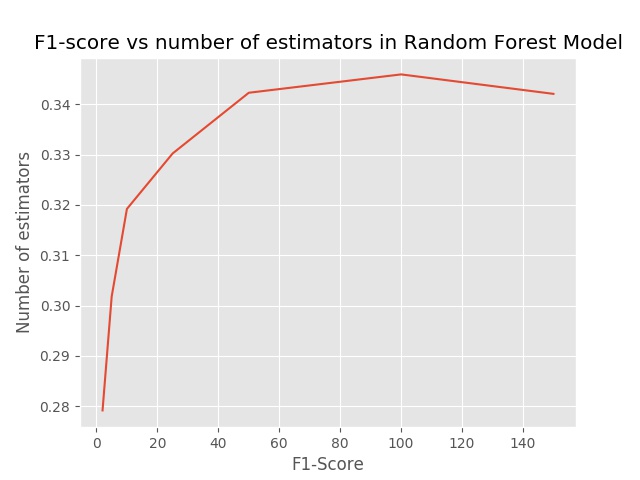
However, since using Decision Tree models just like this one prone to overfitting and not very common in the real world (or so I have heard) we didn’t stop here. Instead, we took our modeling one step further and used the tuned Decision Tree hyperparameters as input for a Random Forest classifier which creates multiple trees from subsets of our data to make many weaker predictions that we then can combine using majority voting to get our final classification outcome in order increase the stability of our model. Tuning were performed once again with the below candidate parameters and the F1-score for the chosen n_estimator values and by looking at the below plot we could discern that the best value for our n_estimator is 100.
# Candidate parameters for the Random Forest model used in GridSearchCV
forest_param_grid = {"feature_selection__k": [7],
                     "classification__criterion": ["gini"],
                     "classification__min_samples_split": [19],
                     "classification__n_estimators": [2, 5, 10, 25, 50, 100,
                                                      150]}
In machine learning validation used to check a model’s general performance in contrast to its performance on the data used to fit the model initially. This is to simulate how the model would perform using new and unseen data and is an invaluable tool for avoiding overfitting to noise that might only exist in the data used initially for training. Ideally, this means that we split up the data into three sets one training set, one test set, and one validation set. Also, since the way the data is split might affect how the outcome of the valuation repeating this the evaluation over many different splits is also desirable.
Since our data set is rather small we will use our test set for both testing and validation, and as mentioned earlier are labels are unbalanced StratifiedShuffleSplit (also used in the provided tester.py) from sklearn where used to split up our data set into testing and training sets while trying to keep the ratio of POIs and non-POIs from the initial data. To make our validation more robust we split the data multiple times creating 1000 different pairs of training and testing data before performing cross-validation and calculating our performance metrics as means for all 1000 different variations. Running the final model through the provided tester.py to validate our work results in the below output.
Pipeline(memory=None,
        steps=[('feature_selection', SelectKBest(k=7,
                                                 score_func=<function f_classif at 0x107cb4b90>)),
               ('classification', RandomForestClassifier(bootstrap=True,
                                                         class_weight='balanced',
                                                         criterion='gini',
                                                         max_depth=None,
                                                         max_features='auto',
                                                         max_leaf_nodes=None,
                                                         min_impurity_decrease...timators=100,
                                                         n_jobs=1,
                                                         oob_score=False,
                                                         random_state=42,
                                                         verbose=0,
                                                         warm_start=False))])

Accuracy:   0.83687
Precision:  0.40791         Recall: 0.49500
F1:         0.44726         F2:     0.47473

Total predictions:  15000
True positives:     990     False positives:    1437
False negatives:    1010    True negatives:     11563
While our accuracy hasn’t changed that much, focusing on the Precision and Recall values we can see that 40% of our model’s predicted POIs are correct (Precision) while 49% of the POIs existing in the dataset was found successfully (Recall).
As you might have realized reading this post here the subject of machine learning and modeling is much deeper than the other parts of data science and thus to write down every thought and present every line of code would result in something much more demanding than just a single blog post. With the latest breakthroughs in AI it might also be easy to give this part too much focus sacrificing the equally important statistical analysis part of the data analysis cycle. However, I hope to be able to go in deeper into this subject once I am starting to write posts on my own not having the pressure of an external deadline.
Next post will be the last post from my Nanodegree endeavor and looking back it definitely has been an adventure trying to keeps up with both study, work and social life. Even after finishing I think I will have a couple of posts to write regarding the process and tools I have used while studying to see if I can find what suits my work-style for personal projects but from there it is going to be all unexplored terrain again.